🎯 Operational Space Controller (OSC)#

MotrixSim provides an Operational Space Controller (OSC) in the motrixsim.osc module. It exposes a single stateless solver class OscSolver that computes joint torques for task-space end-effector control.

Basic Concepts#

Operational Space Control (OSC) is a torque control method for robot manipulators. Unlike Inverse Kinematics, which computes joint positions to achieve a desired end-effector pose, OSC computes joint torques that account for the robot’s full dynamics (inertia, Coriolis forces, gravity). The computation process can be expressed as: joint_torques = compute_osc(osc_solver, ik_chain, end_effector_goal).

IK Model#

OSC reuses the same IkChain from motrixsim.ik to define the kinematic chain. An IK chain model consists of a series of connected joints and an end-effector, as shown below:

ikchain

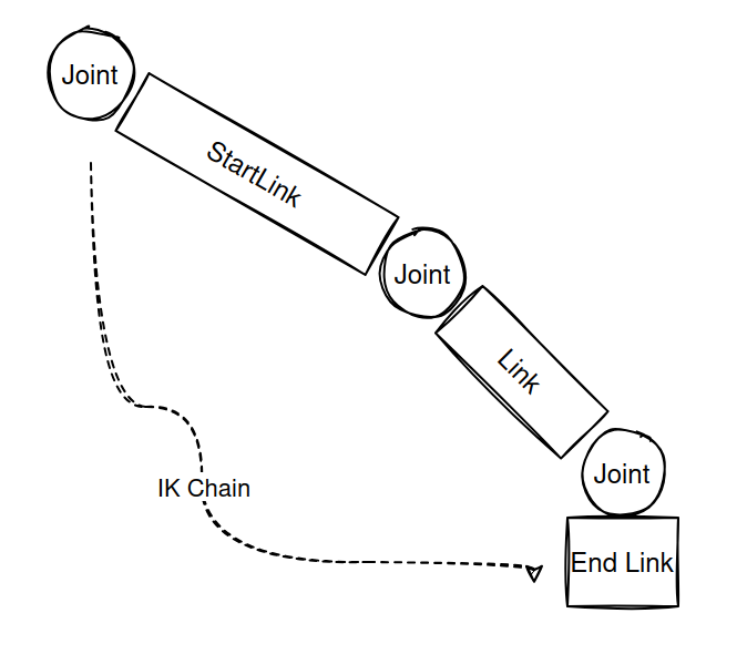
In MotrixSim, you can create an IK chain model as follows:

# Create IK chain for the 7-DOF arm
chain = IkChain(
    model,
    end_link="base",
    start_link="gen3/base_link",
    end_effector_offset=np.array([0.0, 0.0, 0.15, 0, 0, 0, 1], dtype=np.float32),
)

# Create OSC solver (stateless)
solver = OscSolver(
    control_ori=True,
    uncouple_pos_ori=True,
    kp=200.0,
    damping_ratio=1.0,
    nullspace_kp=10.0,
)

The code above creates an IK chain model by specifying the end link and an optional starting link. You can also define the offset of the end-effector relative to the end link using the end_effector_offset parameter.

Refer to the API documentation for more details about IkChain.

OSC Solver#

After defining the IK chain, create an OscSolver to perform the actual torque computation. The solver is stateless — it holds no simulation state. You own the IkChain and the goal variables, updating them as needed each control step.

Constructor parameters:

Parameter	Type	Default	Description
`control_ori`	`bool`	`True`	Enable orientation control in addition to position
`uncouple_pos_ori`	`bool`	`True`	Decouple position and orientation control
`kp`	`float` or `ndarray`	`150.0`	Stiffness gain for tracking the target
`damping_ratio`	`float`	`1.0`	Damping ratio; `1.0` = critically damped (no overshoot)
`nullspace_kp`	`float`	`10.0`	Stiffness gain for nullspace joint position control

Then, compute joint torques by calling the solve method:

# Compute torques using OscSolver (stateless)
torques = solver.solve(chain, goal_pos, goal_ori, nullspace_target, data)

# Check for torque saturation (before clipping)
torque_max_large = np.max(np.abs(torques[:4]))
torque_max_small = np.max(np.abs(torques[4:]))
torque_max = max(torque_max_large, torque_max_small)
torques_saturated = torque_max_large > 105.0 or torque_max_small > 52.0

# Apply torques to arm actuators
# In stanford_tidybot model, the first 3 actuators are for the mobile base (position control),
# actuators 3-9 are for the 7-DOF arm (torque control)
ctrls = data.actuator_ctrls
# Use Kinova Gen3 torque limits: large joints ±105 Nm, small joints ±52 Nm
torques_clipped = np.clip(torques[:4], -105.0, 105.0).tolist() + np.clip(torques[4:], -52.0, 52.0).tolist()
ctrls[3:10] = torques_clipped
data.actuator_ctrls = ctrls

# Step simulation AFTER applying controls
step(model, data)

The solve method returns a numpy.ndarray of shape (*data.shape, num_dof) containing the computed joint torques. You are responsible for applying these torques to the correct actuator indices in data.actuator_ctrls.

solve parameters:

Parameter	Shape	Description
`chain`	—	`IkChain` defining the kinematic chain
`ee_target_pos`	`(*data.shape, 3)`	Target end-effector position `[x, y, z]` in world frame
`ee_target_ori`	`(*data.shape, 3)`	Target orientation as axis-angle `[ax, ay, az]` (direction = rotation axis, magnitude = angle in radians)
`nullspace_joint_pos`	`(*data.shape, num_dof)`	Reference joint positions for nullspace control
`data`	—	Current `SceneData` (supports batched multi-world simulation)

Parameter tuning:

kp — stiffness gain

Controls how aggressively the controller tracks the target. Higher values produce faster response but may cause oscillation or torque saturation.

Small values (50–100): Soft, compliant behavior
Medium values (150–200): Good balance for most applications, recommended starting point
Large values (200–400): Stiff, fast tracking; watch for torque saturation

damping_ratio

Controls the velocity damping relative to kp.

1.0: Critically damped — recommended starting point, no overshoot
< 1.0: Underdamped — faster but may oscillate
> 1.0: Overdamped — slower but very stable

nullspace_kp

Drives joints toward nullspace_joint_pos without disturbing the end-effector task. Useful for keeping redundant joints away from limits. Set to 0.0 to disable. Typical range: 5–20.

Note

When using the OSC Solver, you may encounter instability or poor tracking. Possible reasons include:

The target position is outside the robot arm’s reachable workspace.
Torques saturate at actuator limits — reduce kp or increase damping_ratio.
The robot is near a singular configuration — reduce kp or move the robot away from the singularity.

Tips for better performance:

Start with kp = 150.0 and damping_ratio = 1.0, then tune from there.
Initialize nullspace_joint_pos to the robot’s home configuration to keep joints away from limits.
For batched (multi-world) simulation, all inputs must have a leading batch dimension matching data.shape.
The solver computes torques for the chain’s DOF only — map them to the correct indices in data.actuator_ctrls (see the example).

See the complete code in examples/osc.py