🦾 Inverse Kinematics (IK)#
MotrixSim provides an efficient and easy-to-use Inverse Kinematics (IK) solver located in the motrixsim.ik module. It supports two IK solvers: a Gauss-Newton-based solver (GaussNewtonSolver) and a Damped Least Squares (DLS) solver (DlsSolver), along with a simple IK chain model (IkChain).
Basic Concepts#
Inverse Kinematics (IK) is the process of calculating the joint parameters required to achieve a specific position and orientation of a robot’s end-effector (e.g., a robotic arm’s gripper). In contrast, Forward Kinematics calculates the position and orientation of the end-effector based on known joint parameters. The IK computation process can be expressed as: joint_dof_pos = compute_inverse_kinematic(ik_model, end_effector_pose).
IK Model#
The IK model defines the structure and constraints of the IK problem. Currently, MotrixSim only supports chain structures (IKChain) composed of single-degree-of-freedom joints (Hinge, Slide).
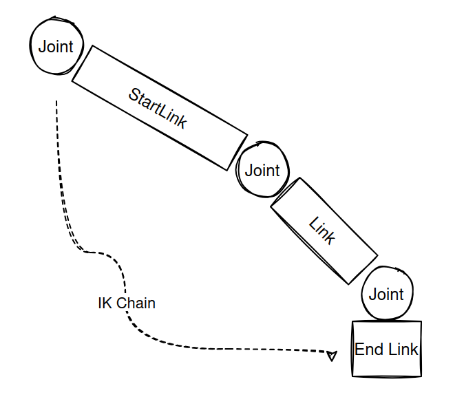
IK Chain#
An IK chain model consists of a series of connected joints and an end-effector, as shown below:
In MotrixSim, you can create an IK chain model as follows:
chain = ik.IkChain(
    model, end_link="base", start_link="gen3/base_link", end_effector_offset=[0.0, 0.0, 0.15, 0, 0, 0, 1]
)
assert chain.num_dof_vel == 7, f"Expected 7 DoF for the Stanford TidyBot arm, got {chain.num_dof_vel}"
The code above creates an IK chain model by specifying the end link and an optional starting link. You can also define the offset of the end-effector relative to the end link using the end_effector_offset parameter.
Refer to the API documentation for more details about IkChain.
IK Solver#
After defining the IKModel, you can use an IK Solver to perform the actual IK solving. MotrixSim supports two IK solvers: the traditional Gauss-Newton solver GaussNewtonSolver and the more robust Damped Least Squares (DLS) solver DlsSolver.
Damped Least Squares (DLS) IK Solver#
The Damped Least Squares (DLS) method is a robust optimization algorithm that adds regularization to handle singular configurations and improve numerical stability. It’s particularly effective when dealing with near-singular Jacobian matrices or when the robot arm approaches singular configurations. DLS is also known as the Levenberg-Marquardt method when applied to IK problems.
Key advantages:
Better numerical stability near singular configurations
More consistent convergence behavior
Adjustable damping parameter for different scenarios
In MotrixSim, you can create a DLS IK solver as follows:
# Damped Least Squares (DLS) solver with robust numerical stability
solver = ik.DlsSolver(
    max_iter=100,
    step_size=0.5,
    tolerance=1e-3,
    damping=1e-3,  # Key parameter for DLS - start with 1e-3 for most applications
)

# Alternative: use Gauss-Newton solver (faster but less stable near singularities)
# solver = ik.GaussNewtonSolver(
#     max_iter=100,
#     step_size=0.5,
#     tolerance=1e-3,
# )

# DLS Damping parameter tuning guide:
# - damping=1e-5: Near Gauss-Newton behavior, fast convergence when well-conditioned
# - damping=1e-3: Good balance for most applications (default)
# - damping=1e-1: Very stable but slower, useful near singular configurations
Damping Parameter Tuning: The damping parameter is crucial for DLS performance:
Small values (1e-6 to 1e-4): Near Gauss-Newton behavior, fast convergence when well-conditioned
Medium values (1e-4 to 1e-2): Good balance for most applications, recommended starting point
Large values (1e-2 to 1.0): More stable but slower convergence, useful near singularities
Gauss-Newton IK Solver#
The Gauss-Newton method is an iterative optimization algorithm for nonlinear least squares problems. It linearizes the nonlinear function and uses the least squares method to update parameter estimates, gradually approaching the target value. In IK solving, the Gauss-Newton method iteratively adjusts joint parameters to make the end-effector’s position and orientation as close as possible to the target position and orientation.
The Gauss-Newton solver is simpler and may converge faster when the system is well-conditioned, but can struggle near singular configurations.
When to use DLS vs Gauss-Newton:
Use DLS when working near singular configurations, when numerical stability is important, or when you encounter convergence issues with Gauss-Newton
Use Gauss-Newton when you need maximum speed and the system is well-conditioned, away from singularities
Then, execute the IK solving process by calling the solve method:
result = solver.solve(chain, data, target_pose)
# the first element is actual iteration number used, which may be less than max_iter
num_iter = result[0]  # noqa: F841
# the second element is the final residual after iteration end.
residual = result[1]
# the remaining elements are the desired dof_pos
desired_dof_pos = result[2:]

# Check convergence: residual < tolerance means successful convergence
if residual < 1e-3:
    # in stanford_tidybot model, the first 3 actuators are for the mobile base,
    # we only need to control the arm dof_pos.
    ctrls = data.actuator_ctrls
    ctrls[3:10] = desired_dof_pos
    data.actuator_ctrls = ctrls
else:
    # DLS typically provides better convergence than Gauss-Newton,
    # but if you still see convergence issues, try:
    # 1. Increasing damping parameter (e.g., 1e-2)
    # 2. Breaking down large movements into smaller steps
    # 3. Checking if target is within robot workspace
    print(f"IK not converged: iterations={num_iter:.0f}, residual={residual:.2e}")
    print("Tips: increase damping, use smaller steps, or check workspace limits")
The solve method returns a numpy.ndarray object with the shape (*data.shape, chain.num_dof_pos + 2), where chain.num_dof_pos is the number of degrees of freedom in the IK chain. The additional two elements represent the solver’s convergence status and the number of iterations.
Note
When using the IK Solver, it may sometimes fail to converge. Possible reasons include:
The target position is outside the robot arm’s workspace.
The IK process does not consider constraints such as collisions.
The initial pose of the robot arm is too far from the target, making it impossible to converge within the set number of iterations.
For Gauss-Newton: The system is near a singular configuration where the Jacobian matrix becomes ill-conditioned.
For DLS: The damping parameter might need adjustment for your specific use case.
Tips for better convergence:
Use DLS solver when working near singular configurations
Adjust the damping parameter based on your scenario (start with 1e-3)
Ensure the target pose is reachable within the robot’s workspace
Consider breaking down large movements into smaller incremental steps
See the complete code in examples/ik.py