🦾 反向运动学(IK)#
MotrixSim 提供了一个高效且易于使用的反向运动学(IK)求解器,位于motrixsim.ik模块中。
它支持两种 IK 求解器:基于高斯-牛顿法的求解器(GaussNewtonSolver)和阻尼最小二乘法(DLS)求解器(DlsSolver),以及简单的 IK 链模型(IkChain)。
基本概念#
Inverse Kinematics (IK) 是计算机器人末端执行器(如机械臂手爪)位置和姿态所需的关节参数的过程。与之相对的是正向运动学(Forward Kinematics),它是通过已知的关节参数来计算末端执行器的位置和姿态。
用一个公式来表示 IK 计算过程就是: joint_dof_pos = compute_inverse_kinematic(ik_model, end_effector_pose)。
IK Model#
IK 模型用于定义 IK 问题的结构和约束。当前 MotrixSim 仅支持由单自由度关节(Hinge,Slide)组成的链式结构(IKChain)。
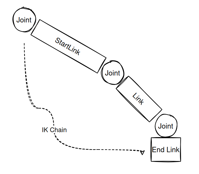
IK Chain#
IK 链模型由一系列连接的关节和一个末端执行器组成, 如下图所示:
在 MotrixSim 中,您可以通过以下方式创建一个 IK 链模型:
chain = ik.IkChain(
    model, end_link="base", start_link="gen3/base_link", end_effector_offset=[0.0, 0.0, 0.15, 0, 0, 0, 1]
)
assert chain.num_dof_vel == 7, f"Expected 7 DoF for the Stanford TidyBot arm, got {chain.num_dof_vel}"
以上代码通过指定末端连杆和可选的起始连杆来创建一个 IK 链模型。您还可以通过 end_effector_offset 参数来定义末端执行器相对于末端连杆的偏移。
您可以查看 API 文档了解更多关于 IkChain 的信息。
IK Solver#
在定义了 IKModel 之后,您可以使用 IK Solver 来做具体的 IK 求解工作。MotrixSim 支持两种 IK 求解器:传统的高斯-牛顿法求解器(GaussNewtonSolver)和更稳定的阻尼最小二乘法(DLS)求解器(DlsSolver)。
阻尼最小二乘法(DLS)IK 求解器#
阻尼最小二乘法(DLS)是一种鲁棒的优化算法,它通过添加正则化项来处理奇异配置并提高数值稳定性。当处理接近奇异的雅可比矩阵或机械臂接近奇异配置时,DLS 特别有效。DLS 在 IK 应用中也被称为 Levenberg-Marquardt 方法。
主要优势:
在奇异配置附近具有更好的数值稳定性
更一致的收敛行为
针对不同场景可调节的阻尼参数
在 MotrixSim 中,您可以通过以下方式创建 DLS IK 求解器:
# Damped Least Squares (DLS) solver with robust numerical stability
solver = ik.DlsSolver(
    max_iter=100,
    step_size=0.5,
    tolerance=1e-3,
    damping=1e-3,  # Key parameter for DLS - start with 1e-3 for most applications
)

# Alternative: use Gauss-Newton solver (faster but less stable near singularities)
# solver = ik.GaussNewtonSolver(
#     max_iter=100,
#     step_size=0.5,
#     tolerance=1e-3,
# )

# DLS Damping parameter tuning guide:
# - damping=1e-5: Near Gauss-Newton behavior, fast convergence when well-conditioned
# - damping=1e-3: Good balance for most applications (default)
# - damping=1e-1: Very stable but slower, useful near singular configurations
阻尼参数调优指南: 阻尼参数对 DLS 性能至关重要:
小值(1e-6 到 1e-4):接近高斯-牛顿行为,在条件良好时收敛快速
中值(1e-4 到 1e-2):大多数应用的良好平衡点,推荐的起始值
大值(1e-2 到 1.0):更稳定但收敛较慢,在奇异点附近使用
Gauss-Newton IK Solver#
高斯-牛顿法是一种用于非线性最小二乘问题的迭代优化算法。它通过线性化非线性函数并使用最小二乘法来更新参数估计,从而逐步逼近目标值。在 IK 求解中,高斯-牛顿法通过迭代调整关节参数,使得末端执行器的位置和姿态尽可能接近目标位置和姿态。
高斯-牛顿求解器更简单,在系统条件良好时可能收敛更快,但在奇异配置附近可能会遇到困难。
何时使用 DLS vs Gauss-Newton:
使用 DLS:当在奇异配置附近工作、数值稳定性很重要时,或当您遇到高斯-牛顿的收敛问题时
使用 Gauss-Newton:当您需要最大速度且系统条件良好、远离奇异点时
然后通过调用 solve 方法来执行 IK 求解:
result = solver.solve(chain, data, target_pose)
# the first element is actual iteration number used, which may be less than max_iter
num_iter = result[0]  # noqa: F841
# the second element is the final residual after iteration end.
residual = result[1]
# the remaining elements are the desired dof_pos
desired_dof_pos = result[2:]

# Check convergence: residual < tolerance means successful convergence
if residual < 1e-3:
    # in stanford_tidybot model, the first 3 actuators are for the mobile base,
    # we only need to control the arm dof_pos.
    ctrls = data.actuator_ctrls
    ctrls[3:10] = desired_dof_pos
    data.actuator_ctrls = ctrls
else:
    # DLS typically provides better convergence than Gauss-Newton,
    # but if you still see convergence issues, try:
    # 1. Increasing damping parameter (e.g., 1e-2)
    # 2. Breaking down large movements into smaller steps
    # 3. Checking if target is within robot workspace
    print(f"IK not converged: iterations={num_iter:.0f}, residual={residual:.2e}")
    print("Tips: increase damping, use smaller steps, or check workspace limits")
solve 方法返回 numpy.ndarray 对象,其形状为(*data.shape, chain.num_dof_pos + 2). 其中 chain.num_dof_pos 是 IK 链的自由度数量,额外的两个元素分别表示求解器的收敛状态和迭代次数。
备注
IK Solver在进行求解时,可能会遇到无法收敛的情况,原因是多样的,例如:
目标位置超出了机械臂的工作空间
IK过程并没有考虑碰撞等限制
机械臂的初始姿态距离目标位置过远,无法在设定的迭代次数内收敛
对于高斯-牛顿法:系统接近奇异配置,雅可比矩阵变得病态
对于 DLS:阻尼参数可能需要根据您的具体应用场景进行调整
提高收敛性的技巧:
在奇异配置附近使用 DLS 求解器
根据您的场景调整阻尼参数(从 1e-3 开始)
确保目标姿态在机器人工作空间内可达
考虑将大的运动分解为更小的增量步骤
查看完整代码请见 examples/ik.py