

🚀 Quick Start: Hello MotrixSim#
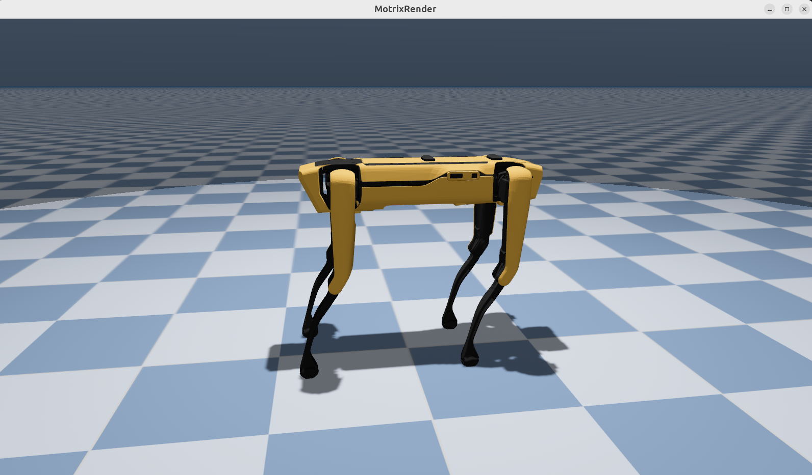
This tutorial demonstrates a simple example—loading the Spot quadruped robot and running a physics simulation—to introduce the core steps and basic concepts for creating simulation experiments in MotrixSim:
import time

import motrixsim as mx

model = mx.load_model("examples/assets/boston_dynamics_spot/scene.xml")
with mx.render.RenderApp("warn") as render:
    render.launch(model)
    data = mx.SceneData(model)

    while True:
        time.sleep(model.options.timestep)
        mx.step(model, data)
        render.sync(data)
That’s the complete code! With just 10 lines, you accomplish all the essential steps for a MotrixSim simulation experiment.
You can now start exploring MotrixSim, or continue reading below for a detailed explanation of each step:
Load the Model#
model = mx.load_model("examples/assets/boston_dynamics_spot/scene.xml")
First, we call load_model to load a model file, which includes both physical and rendering data (see SceneModel for details).
MotrixSim supports multiple model formats, including MJCF and URDF (OpenUSD is under development). Here, we use the MJCF format for the Go1 quadruped robot model, which you can find at examples/assets/boston_dynamics_spot/scene.xml.
You can also use load_mjcf_str to load a model directly from an MJCF string; see examples/load_from_str.py for an example.
Launch the Renderer#
render = mx.render.RenderApp()
Next, we create a renderer instance RenderApp, which is responsible for visualizing the model.
Load the Model into the Renderer#
render.launch(model)
The renderer needs to load the model data before rendering. We call render.launch(model) to start the renderer and load the model.
Create Physics Data (SceneData)#
data = mx.SceneData(model)
Physical simulation requires a data structure to store the model’s state. We use SceneData to create a physics data object associated with the model. This can be considered an instance of the model, and you can create multiple instances from the same model.
Physics Simulation#
mx.step(model, data)
The core of the simulation is the step function, which updates the model’s state. Each call performs a single simulation time step.
In this example, we call step 1000 times in a loop, pausing for 2 milliseconds between each call (the default time step for the go1 model) to simulate the passage of time.
Synchronize the Renderer#
render.sync(data)
After each simulation step, we need to synchronize the model state with the renderer to update the visualization. We call sync to perform this operation.
Note
The call frequency between step and sync does not have to be 1:1. You can adjust the frequency as needed for your application.
With this, the entire example is complete. You can now try modifying parameters to observe the physical effects under different settings.
Next Steps#
See mjcf for supported features
Learn how to use the main features
Explore more example programs